Reliable Digital Oscilloscope for Accurate Signal Analysis

When a signal disappears between two probe points, the difference between a quick fix and a long night often comes down to one thing: how much you trust your oscilloscope. For engineers who need precise, repeatable measurements without second-guessing every trigger event, a reliable digital oscilloscope isn’t just a tool—it’s a lifeline. That’s where TPS comes in, with instruments built to deliver the accuracy that modern signal analysis demands.

Clean Front-End Design Keeps Noise Low and Waveforms Honest

A clean front end starts with a low-noise analog buffer placed as close to the input connector as possible. That placement keeps trace inductance and stray capacitance from filtering the signal before it reaches the ADC. The chosen parts are not exotic; they are simply run in a way that avoids thermal drift and parasitic oscillation.

The board separates the analog ground plane from the digital return path with a single tie point. This keeps high-frequency switching currents out of the sensitive input stage, so the noise floor does not rise when the display or processor is active. The benefit shows up most clearly on low-level signals, where a few millivolts of noise can otherwise swamp the detail.

Waveform fidelity is checked under real loads, not just with a resistive terminator. Capacitive loading, long probes, and fast edges all stress the front end; the design compensates without adding peaking. The result is a trace that matches the signal edges closely, with no artificial rounding or ringing introduced by the input stage.

Trigger Modes That Catch Intermittent Faults, Not Just Repetitive Waves

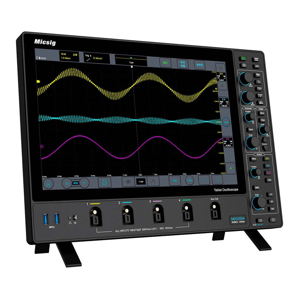
Most oscilloscopes default to edge triggering, which works fine when you're looking at a steady clock or a clean repetitive waveform. But real-world glitches rarely announce themselves on schedule. Intermittent faults—like a dropped pulse, a metastable state, or a bus contention that happens once every few thousand cycles—can slip right past a basic trigger. That's why advanced trigger modes matter: they let you arm the scope to wait for a specific anomaly rather than just syncing to the next rising edge.

Pulse-width triggering, for instance, fires only when a pulse is either too narrow or too wide compared to a user-defined window. Runt triggering catches signals that cross one logic threshold but fail to reach the other—classic signs of bus fights, slow rise times, or insufficient drive strength. Setup-and-hold triggering watches the relationship between a clock and data line, flagging violations that occur sporadically under thermal or voltage stress. Logic triggering extends this idea to multiple channels, letting you qualify the trigger on a pattern that may occur only under a specific combination of inputs.

The real advantage is time. Instead of staring at a screen for hours hoping to see a rare event, you set the trigger condition, go work on something else, and come back to a captured waveform when the anomaly finally happens. That turns intermittent debugging from a passive waiting game into an active hunt—and it's often the only practical way to isolate faults that don't show up in steady-state testing.

Deep Capture Memory Holds the Full Story of Every Signal

Most capture systems only keep the highlights, the obvious peaks that demand attention. Deep capture memory works differently. It refuses to discard the quiet, the transitional, the nearly invisible. Every pulse, every dip, every odd little echo gets stored in its original order and shape. The result isn't a summary—it's the complete narrative, from the first flicker to the final fade.

This approach matters because signals rarely announce themselves upfront. A subtle drift in timing or a barely noticeable variance in amplitude might look like noise today but turn out to be the signature of something important tomorrow. Deep capture memory preserves that possibility. It doesn't compress the story into a few convenient data points. Instead, it lets you rewind and zoom into any moment, confident that nothing was trimmed away for the sake of storage space or processing speed.

The practical payoff shows up when you need to answer a question nobody thought to ask before. Why did that anomaly appear? What happened in the milliseconds before the trigger? With deep capture memory, those answers are already waiting—not reconstructed from fragments, but read from the original, uninterrupted record. It's the difference between a sticky note and a transcript. One reminds you of the event. The other lets you live through it again, frame by frame.

Fast Waveform Updates Reveal Anomalies Before They Vanish

When a signal glitch lasts only a few microseconds, a scope that updates slowly will simply miss it. Fast waveform updates change that by redrawing the display thousands of times per second, so intermittent faults appear on screen long enough to be spotted. The key is not just speed for its own sake, but the higher probability of catching a rare event before it disappears into the next acquisition cycle.

This matters most in debugging tasks where the problem is not continuous. A power supply dropout, a metastable logic state, or a jitter spike may occur once in every ten thousand triggers. With a sluggish update rate, those anomalies flicker past between screen refreshes and never register. A fast update engine, however, keeps the display densely populated with fresh acquisitions, turning a near-invisible event into something you can actually see and then isolate with deeper triggering.

Engineers often overlook how much visual persistence affects their workflow. When the waveform update rate is high, the scope builds an intensity gradient that highlights outliers, so the rare anomaly stands out against the normal trace instead of being buried in a single static capture. That visual cue is often the first step toward narrowing down the root cause.

Stable Calibration Across Temperature Shifts and Long Sessions

Calibration drift is the quiet killer of reliable measurement. Many devices behave perfectly during a short bench test, yet shift noticeably once the ambient temperature moves by ten degrees or the unit has been running for six hours straight. This isn't just a nuisance — it's a failure of the underlying reference and compensation architecture. To keep readings trustworthy across thermal swings and marathon operating periods, the design must treat stability as a first-class requirement, not an afterthought.

A practical approach starts with choosing references and front-end components whose temperature coefficients and long-term aging profiles are well characterized, then pairing them with a compensation loop that runs continuously. Instead of a one-time factory trim, the system periodically samples known internal reference points and adjusts for drift in real time. This dynamic correction, combined with modest thermal shielding and careful board layout to avoid hot spots, keeps the error budget flat even as conditions change around the instrument.

Long sessions introduce their own stress: cumulative heating, component relaxation, and slow supply voltage wander. Here, the goal is not just to survive a 24-hour run, but to show no meaningful difference between minute five and hour twenty. By tracking drift residuals and using a lightweight adaptive model, the system can anticipate small shifts before they exceed tolerance. The result is a calibration that holds its shape — whether the lab is cold in the morning or the equipment has been logging data through the night.

Straightforward Connectivity for Lab Benches and Field Work

Most lab instruments still rely on a tangle of cables and adapters that seem designed to trip you up halfway through an experiment. Our approach cuts through that. Every port on the bench unit is clearly labeled and color-coded, so you can swap sensors or power sources without hunting for a manual. The same logic carries into the field: ruggedized connectors click into place with an audible snap, and there’s no fiddly alignment required, even with gloves on.

Wireless pairing is available but never forced. When a cable makes more sense—say, for high-throughput data or a long-duration run—you get a locking USB-C connection that won’t wobble loose. In the field, Bluetooth Low Energy keeps tablets and phones linked for quick readouts, while an optional long-range radio module handles sites where Wi-Fi doesn’t reach.

Setup time drops from minutes to seconds because the system remembers your last configuration. Plug in a probe and the interface auto-detects it, pulling up the right calibration curve and unit preferences. That kind of continuity between lab bench and field kit means you spend less energy on hookup logistics and more on the actual work.

FAQ

Conclusion

A truly reliable digital oscilloscope does not earn that label through a single headline specification. It comes from the way the front-end treats the signal before it ever reaches the display. The clean input design keeps the noise floor low, so what you see is the actual waveform rather than a haze of pickup and distortion. That matters more than most spec sheets admit, because a quiet front-end means small signal details survive long enough to be measured. On top of that, the trigger system is built for real troubleshooting: it catches intermittent faults like runt pulses, glitches, or timing violations that an ordinary edge trigger would skip. When a rare event fires, the deep capture memory holds the entire signal story at full sample rate, so you can zoom in after the fact and still see the exact transition that caused the failure.

Fast waveform updates also change how you work. Instead of staring at one frozen capture, the display refreshes thousands of times per second, revealing anomalies that pop in and out before they vanish. Calibration stability keeps those measurements dependable over long sessions and across temperature shifts, so a rising lab temperature does not quietly skew your amplitude or timebase. Finally, connectivity is straightforward whether you are on a lab bench or in the field: data export, remote control, and instrument sync happen without cumbersome setup. None of these features alone makes the scope reliable; it is the way they work together that turns raw acquisition into accurate signal analysis.